The Big Problem is Medium Data


This is a guest post by Matt Hunt, who leads open source projects for Bloomberg LP R&D.
“Big Data” systems continue to attract substantial funding, attention, and excitement. As with many new technologies, they are neither a panacea, nor even a good fit for many common uses. Yet they also hold great promise. The question is, can systems originally designed to serve hundreds of millions of requests for something like web pages also work for requests that are computationally expensive and have tight tolerances?
Modern era big data technologies are a solution to an economics problem faced by Google and other Internet giants a decade ago. Storing, indexing, and responding to searches against all web pages required tremendous amounts of disk space and computer power. Very powerful machines, fast SAN storage, and data center space were prohibitively expensive. The solution was to pack cheap commodity machines as tightly together as possible with local disks.
This addressed the space and hardware cost problem, but introduced a software challenge. Writing distributed code is hard, and with many machines comes many failures. So a framework was also required to take care of such problems automatically for the system to be viable.
Hadoop
Right now, we’re in a transition phase in the industry in computing built from the entrance of Hadoop and its community starting in 2004. Understanding why and how these systems were created also offers insight into some of their weaknesses.
At Bloomberg that we don’t have a big data problem. What we have is a “medium data” problem -- and so does everyone else. Systems such as Hadoop and Spark are less efficient and mature for these typical low latency enterprise uses in general. High core counts, SSDs, and large RAM footprints are common today - but many of the commodity platforms have yet to take full advantage of them, and challenges remain. A number of distributed components are further hampered by Java, which creates its own complications for low latency performance.
A practical use case
“Medium data” refers to data sets that are too large to fit on a single machine but don’t require enormous clusters of thousands of them: high terabytes, not petabytes.
So, let’s take a practical use case from Bloomberg around times series data and the issues we had with speed and volume. Time series data for a security is generally just a security (i.e. IBM), a field (i.e. price), a date and a value.
These systems have also historically been separated into intraday and historical data – intraday captures all the ticks during the day, while historical systems have end-of-day values that go back much farther in time. Unifying them was impractical in the past because of different performance tradeoffs: intraday must manage a very high volume of incoming writes, while end-of-day has batch updates on market close, but more data and searches in total.
The response time for a year’s data for a field on a security is 5 milliseconds, and it receives billions of hits a day, around half a million a second at peak. It is a critical system for Bloomberg; failures there have the potential to disrupt the capital markets.
The challenge then comes from applications like Portfolio Analytics that request far more data at a time. A bond portfolio can easily have tens of thousands of bonds in it, and a common calculation like attribution requires 40 fields per day per instrument. Performing attribution for a bond portfolio over a few years of data requires tens of millions of datapoints instead of a handful. When requesting tens of millions of datapoints, even a high cache hit rate of 99.9% will still have thousands of cache misses, and if the underlying system is backed by magnetic media, this means thousands of disk seeks. Multiply across a large user base making many requests and it’s clear to see why this created a problem for the existing price history system.
The solution a few years back was to move to all memory and solid state machines with highly compacted blobs split into separate databases. This approach worked and was 2-3 orders of magnitude faster – a giant leap – but less than ideal. Compacted blobs split across many databases is cumbersome.
Time series data is both very simple and lends itself to embarrassing parallelism. When fetching tens of millions of datapoints for a portfolio, the work can be arbitrarily divided among tens of millions of machines if need be. It doesn’t get any better than that in terms of potential parallelism. With a single main table trivially distributed, Hbase should be a good fit – in theory.
Of course in theory, theory and practice agree. But in practice, that is not always the case. The data sets may work, but there are obstacles including performance, efficiency, maturity, and resiliency. What follows is how we went about tackling those obstacles.
When an individual machine fails, data is not lost – it is replicated on several machines via HDFS – but there is still a serious drawback. At any given time, all reads and writes to any given region is managed by one and only one region server. If a region server dies, the failure will be detected and a replacement automatically brought back up, but until it does, no reads and writes are possible to the regions it managed.
The Hbase community has made great strides in speeding up recovery time after a failure is detected, but this still leaves a crucial hole. The crux of the problem is that failure detection in a distributed system is ultimately accomplished by timeout – some period of time that elapses where a heartbeat or other mechanism fails. If this timeout is made too short, there will be false positives, which are also problematic.
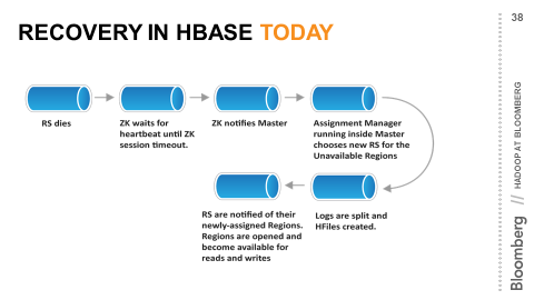
In Bloomberg’s case, our SLA’s are on the order of milliseconds. The shortest that timeouts can be made are on the order of many seconds. This is a fundamental mismatch even if recovery after failure detection becomes infinitely fast.
Discussions with Hadoop vendors resulted in several possible solutions, most of which involved running multiple copies of each database. Since Bloomberg’s operational policies already dictate that systems can survive the loss of entire datacenters and then several additional machines, this would have meant many running copies of each database, which we deemed too operationally complex. Ultimately, we were unhappy with the alternatives, and so we worked to change them.
If failover detection and recovery can never be fast enough, then the alternative is there must be standby nodes that can be queried in the event a region server goes down. The insight that made this practical in the short term is that the data already exists in multiple places, albeit with a possible slight delay in propagation, but that this can be used for standby region servers that at worst lag slightly behind but receive events in the same order, providing timeline consistency, which works for end of day systems like price history that are updated in batch.
Timeline consistent standby region servers were added to Hbase as part of JIRA-10070.
Conclusion and next steps
HBase has a number of other obstacles to performance other than failover. Careful examination of the source of bottlenecks allowed us to increase the speed dramatically by using careful key selection, in-place computation, and techniques such as synchronized garbage collection.
By employing this approach, we’ve found extraordinary performance improvements, namely:
PORT write performance 1000x faster
Read retrieval is about 3x as fast as previous rate
With HBase experiments, we can cut average runtime response times to a quarter of what they were, with plenty of room left for further improvements. Faster machines are available that would halve response times again. By developing on an open source system and being conscientious of our vendor choices, we were able to see some great results in performance for our medium data problem.
More importantly, our goal is more than performance alone. While this setup with HBase provides a thousandfold improvement on write performance and 3x faster reads, it is a connector to a broader distributed platform of tools and ideas.
What do you think? Would your organization be a fit for this kind of implementation? And what questions do you have about the specifics of the experiments?
APPENDIX: DIAGRAMS OF HBASE DISTRUBUTION
Performance I: distribution and parallelism

Performance II: In place computation
With failures addressed, though, there are still issues of raw performance and consistency. Here we’ll detail three experiments and outcomes on performance. Tests were run on a modest cluster of 11 machines with SSDs, dual Xeon E5’s, and 128GB of RAM each. In the top right hand corner of the slide, two numbers are shown. The first is the average response time at the outset of the experiment, and the second the new time after improvements were made. The average request is for around 200,000 records that are random key-value lookups.
Part of the premise of HBase is that large Portfolio requests can be divided up and tackled among existing machines in a cluster. This is part of why standby region servers to address failures are mandated – if a request hits every server, and one doesn’t respond for a minute or more, it’s bad news. The failure of any one server would stall every such request.
So the next thing to tackle was parallelism and distribution. The first issue was in dividing work evenly: given a large request, did each machine in the cluster get the same size chunk of work? Ideally, requesting 1000 rows from ten machines would get 100 rows from each. With a naïve schema, the answer is no: if the row key is security + something else, then everything from IBM will be in one region, and IBM is hit more often than other securities. This phenomena is known as hotspotting.
The solution is to take advantage of the properties of HBase to fix. Data in HBase is always kept physically sorted by the row key. If the row key itself is hashed, and that hash used as a prefix, then the rows will be distributed differently. Imagine the rowkey is security+year+month+field. Take an MD5 of that, and use that as a prefix, and any one record for IBM is equally likely to be on any server.
This resulted in almost perfect distribution of work load. We didn’t use MD5, because it’s too slow and large, but the concept is the same.
With perfect distribution, we have perfect parallelism: with 11 servers each one was doing the same amount of work not just on average, but for every request. And if parallelism is good, then more parallelism is better, right? Yes - up to a point.
As mentioned earlier a general Hadoop weakness is that it was designed for older and less powerful machines. One of the ways this manifests itself is through low resource consumption on the server. At maximum throughput, none of the hardware was breathing hard – low cpu and disk and network, no matter how many configuration options were changed.
One way to address this is to run more region servers per machine, provided the machine has the capacity to do so. This will increase the number of total region servers and hence the level of fan out for parallelism, and if more parallelism is better, then response times will drop.
The chart from the slide shows the results. With 11 machines and 1 region server each – 11 in total – average response time was 260ms. Going to 3 per machine, for 33 region servers in total, dropped the average time to 185ms. 5 region servers per machine further improved to 160ms, but at 10 per machine times got worse. Why?
The first answer that will probably spring to mind is that the capacity of the machine was exceeded; with 10 region server processes on a box, each with many threads, perhaps there weren’t enough cores. As it turns out, this is not the cause, and the actual answer is more subtle and interesting and resulted in another leap in performance that is applicable to many systems of this type.
But before we get into that, let’s talk about in place computation.
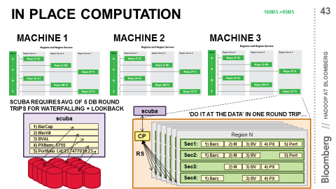
One of the tenets of big data is that the computation should be moved to the data and not the other way around. The idea here is straightforward. Imagine you need to know how many rows are in a large database table. You could fetch every row to your local client, and then iterate through and count – or you could issue a “select count(*) from… “ if it’s a relational database. The latter is much more efficient.
It’s also much more easily said than done. Many problems can’t be solved this way at all, and many frameworks fall short even where the problem is known to be amenable. In the 2013 report on massive data analysis the National Research Council proposed 7 computational giants for parallelism in an attempt to categorize the capabilities of a distributed system, a relevant and interesting read, and Hadoop can’t handle all of them.
Fortunately for us, we have a simple use case that does make sense that let us again cut response times in half.
The situation is that there are multiple “sources” for data. Barclays and Merrill Lynch and many other companies provide data for bond pricing. The same bond for the same dates is often in more than one source, but the values don’t agree. Customers differ on the relative precedence of each, and so with each request include a waterfall which is just an ordering of what sources should be used in what order. Try to get all the data from the first source, and then for anything that’s missing, try the next source , and so on. On average, a request must go through 5 such sources until all the data is found.
In the world of separate databases, different sources are in different physical locations, and so this means trying the first database, pulling all the records back, seeing what’s missing, constructing a new request, and issuing that.
For HBase, we can again take advantage of physical sorting, support for millions of columns, and in-place computation through coprocessors, which are the HBase equivalent of classic stored procedures.
By making the source and field columns with the security and date still the rowkey, they will all be collocated on the same region server. The coprocessor logic then becomes “find the first source for this row that matches for this security on this date, and return that.” Instead of 5 round trips, there will always be one and only one.
A small coprocessor of a few lines worked as expected, and average response time dropped to 85ms.
Performance III: Synchronized disruption
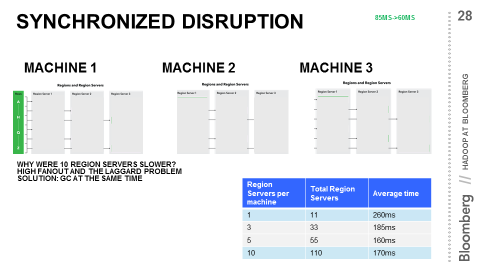
The results from increasing the number of region servers left a mystery: why did response times improve at first, and then worsen? The answer involves both Java and an important property of any high fan out distributed system.
A request that goes to more than one machine “fans out”. The more machines hit, the higher the degree of fan out. In a request that fans out, how long does it take to get a response?
The answer is that it takes as long as the slowest responder. With ten region servers per machines and 11 machines, each request fanned out to 110 processes. If 109 respond in a microsecond and 1 in 170ms, the response time is 170ms.
The immediate culprit turned out to be java garbage collection, which freezes a machine until it completes. The higher the degree of fan-out, the greater the likelihood that any one region server process was garbage collecting at the time. At 110 regions, the odds were close to 1.
The solution here is devilishly simple. As long as the penalty must be paid if any one java process garbage collects, why not just make them do it all at the same time? That way, more time will elapse where requests are issued and no garbage collection takes place. We wrote the simplest, dumbest test for this: a coprocessor with one line – system.gc() – and a timer that called it every 30 seconds.
This dropped our average response time from 85ms to 60ms on the first go.
Many system developers and C programmer eyeballs will collectively roll as this is a Java specific problem. While Java gc is an issue, this has wider applicability. It is a general case of what Google’s Jeff Dean calls Synchronized Disruption. Requests in any parallel system that fan out suffer from the laggard, and so things that slow down individual machines should be done at the same time. For more details, see the excellent writeup “Achieving Rapid Response Times in Large Online Services” covering this and other properties of high fan out systems.
That said, Java is the basis now of quite a number of high fan out computing systems, including Hadoop, HBase, Spark, and SOLR. Synchronizing garbage collection holds potential for them as well.
Related Articles
- Big Data London Meetup Event
- Bloomberg Labs
- Bloomberg on Github