When Should Approximate Query Processing Be Used?


This is a guest repost by Barzan Mozafari, an assistant professor at University of Michigan and an advisor to a new startup, snappydata.io, that recently launched an open source OLTP + OLAP Database built on Spark.
The growing market for Big Data has created a lot of interest around approximate query processing (AQP) as a means of achieving interactive response times (e.g., sub-second latencies) when faced with terabytes and petabytes of data. At the same time, there is a lot of misinformation about this technology and what it can or cannot do.
Having been involved in building a few academic prototypes and industrial engines for approximate query processing, I have heard many interesting statements about AQP and/or sampling techniques (from both DB vendors and end-users):
Myth #1. Sampling is only useful when you know your queries in advance
Myth #2. Sampling misses out on rare events or outliers in the data
Myth #3. AQP systems cannot handle join queries
Myth #4. It is hard for end-users to use approximate answers
Myth #5. Sampling is just like indexing
Myth #6. Sampling will break the BI tools
Myth #7. There is no point approximating if your data fits in memory
Although there is a grain of truth behind some of these myths, none of them are actually accurate. There are many different forms of sampling, approximation, and error quantification, and their nuances are missed by these blanket statements. In other words, many of these impressions are simply based on wrong assumptions and/or misunderstanding of basic AQP terminology.
Anyhow, instead of going over each of these statements and explaining why they are categorically wrong, in this post I’d like to answer the positive question: When can (and should) one use approximate answers? Note that by asking this question, I am implicitly giving away that I don’t think approximate answers are always useful. A perfect example where you don’t want to use approximation is in billing departments. (Although every time I look at my own Internet bill, I start to think that even this example has its own exceptions. I’m too afraid to mention my Internet provider’s name here but I am sure you can guess).
Anyhow, let’s discuss the key reasons and use-cases for approximate answers.
1. Use AQP when you care about interactive response times
I don’t think I need to convince you that there is an insane amount of data being generated, collected, and processed. Everyone agrees that social media, smart phone, online services and more are creating massive volumes of data at unbelievable rates. The part that people often disagree on are the following questions:
A. Does the useful part of this data (a.k.a. working set) fit in memory?
B. Will useful data continue to fit in memory as time goes on?
C. If useful data fits in memory, do we still need to think about approximations?
Question A: In my view, Question A is a ridiculous one to begin with. Instead, we should be asking whether or not it is economical to buy memory that is big enough to hold our entire data set. And the answer to the latter is sometime yes, and sometimes no. For example, at a recent Facebook talk at the University of Michigan, I asked the speaker if the data at Facebook fit in the aggregate memory of their data centers. The answer was that the ratio of the overall data to the total memory size at Facebook was 1 to 10. Of course, Facebook can always buy more memory to cache the rest of their data. But they don’t do it, because it doesn’t make sense for them to spend 10x more money.
Question B: Question B is more interesting. We know that hardware (including memory) is expected to improve (doubled every two years) or get cheaper according to Moore’s law. Data is reported to be growing at the same and or even higher rate than Moore’s law (depending on which categories of data in the IDC report you want to consider). This is significant because if it’s too expensive now to keep our entire data in memory, it will be equally or even more expensive to do so next year. In addition, working-set data will also grow at a similar rate. Here’s a great summary from National Instrument’s Newsletter:
"For every second that the Large Hadron Collider at CERN runs an experiment, the instrument can generate 40 terabytes of data. For every 30 minutes that a Boeing jet engine runs, the system creates 10 terabytes of operations information. For a single journey across the Atlantic Ocean, a four-engine jumbo jet can create 640 terabytes of data. Multiply that by the more than 25,000 flights flown each day, and you get an understanding of the enormous amount of data that exists (Rogers, 2011). That’s “Big Data.”"
Question C: The answer to Question C should be a resounding NO, both for economical reasons as well as technical reasons. The economical reasons are quite obvious: why spend more money on more hardware if you can solve your problem with better (and preferably, free) software? The technical reasons are several: there is serialization and other query processing overheads, concurrent tasks and queries running in the cluster, and most importantly, the need for shuffling intermediate results during query processing. As a result, querying 40GB of fully cached data still takes minutes (sometimes half an hour) on today’s fastest SQL-on-Hadoop engines.
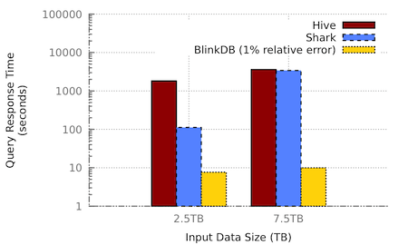
Figure 1 (photo source: this paper) Often a 99% accurate answer can be computed 100-200x faster than an exact answer.
This range of response time is simply unacceptable to many users and applications. Exploratory data analytics is typically an interactive and iterative process: you form an initial hypothesis (e.g., by visualizing and looking at the data), running some queries, modifying your queries based on the previous answers, and so on until you find a satisfactory explanation.
You cannot be productive if you have to wait half an hour every time you run a new query to test a hypothesis. There is a lot of research in the HCI (human-computer interaction) community on how the user’s productivity, engagement, and even creativity is significantly impaired if the computer’s response time exceeds a couple of seconds.*
Because of these reasons there is a fierce competition for providing interactive analytics among commercial and open source data warehouses, including HP Vertica, Amazon’s Redshift, Hive, Impala, Presto, SparkSQL, and many other players. The competition among these different SQL engines is simply about who can implement traditional optimization techniques sooner. These optimizations range from exploiting parallelism, to indexing, materialization, data compression, columnar formats, in-memory and in-situ processing. I am not saying that there is no innovation in this space, but most of the optimizations we hear about (even in the so-called SQL-on-Hadoop solutions) are no different than the mainstream database research on query processing over the past four decades, where the goal is simply one thing:
To efficiently access all relevant tuples to the query while avoiding the irrelevant tuples (e.g., via indexing, materialization, compression, caching)
In a short paper earlier this year I explained that pursuing this goal is not going to be enough. This is because of the rapid growth of data, which is making it increasingly and economically difficult to provide interactive analytics. But the optimization that we are discussing here is of a completely different nature: approximation seems to be the only promising direction in the long run if we have any hopes of delivering interactive response times for Big Data analytics. Instead of processing your entire data, approximation is an optimization that processes only a tiny fraction of your data, but gives you an answer that is extremely close to the true answer that you would have gotten otherwise. For example, most of the time processing 1% of your data might be enough to give you an answer that is 99.9% accurate.
2. Use AQP when you can make Perfect Decisions with Imperfect Answers
In many applications, query results are only useful inasmuch as they enable us to make the best decision. In other words, exact results have no advantage over approximate ones if they both lead to the exact same conclusion/decision. This obviously depends on the quality of your approximation and the application logic. For example, if you work in a billing department, I want you to stop reading the rest of this blog post☺
A/B testing. In marketing and business intelligence, A/B testing is used to refer to a process that compares two variants, A and B. A common application of A/B testing is in ad servers. Ad servers often show two variants of an ad (e.g., with different background colors) to similar visitors at the same time, and measure which variant leads to a higher conversion rate (i.e., more clicks). To find out which variant of the website ad performed better, ad servers need to read through the web server logs, count the number of “clicks” per variant, and normalize by the total number of times each ad variant was displayed. However, the exact click rates for variant A and B, say fA and fB are irrelevant, except that they are needed to decide whether fA > fB or fA < fB. This means that if you can approximate these values such that their relative order is not changed, then you can still perfectly determine which ad variant has been effective. For example, as long as you can infer that 0.1< fA < 0.2 and 0.5< fB < 0.8, you do not care about the exact values of fA and fB.
Hypothesis testing — A major goal of scientific endeavors is to evaluate a set of competing hypotheses and choose the best one. Choosing the best hypothesis often means computing and comparing some effectiveness score for each different hypothesis. For example, the effectiveness score can be the generalization-error (in machine learning), p-values, confidence intervals, occurrence ratios, or the reduction of entropy. Similar to A/B testing, these scores are only useful insofar as they allow for ruling out the unlikely hypotheses. In other words, the scientists do not always need to know the precise value of these scores, as long as they can compare them reliably.
Root cause analysis — Data analysts always seek explanations or the root causes of certain observations, symptoms, or anomalies. Similar to all previous cases, root cause analysis can also be accomplished without having precise information, as long as the unlikely causes can be confidently ruled out.
Exploratory analytics — Data analysts often slice and dice their dataset in their quest for interesting trends, correlations or outliers. If your application falls into this type of explorative analytics, getting an approximate answer within a second is much preferred over an exact answer that takes 20 minutes to compute. In fact, research on human-computer interaction has shown that, to keep your data analyst engaged and productive, the response time of the system must be below 10 seconds. In particular, if the user has to wait for the answer to his/her previous query for more than a couple of seconds, his/her creativity can be seriously impaired.**
Feature selection — One of the factors that usually has the largest impact on the quality of machine learning models is the set of features used for training. This is why a critical step in machine learning workloads is the feature selection step, which consists of choosing a subset of features with the best prediction power. So given N features, there is 2N possible subsets to consider. Again, similar to all the previous use-cases, as long as we can determine that a certain subset is less effective than another, we do not need to compute the exact prediction error of either subsets (see this paper as an example).
Big data visualization — This one is one of my favorite use-cases. Visualization tools have become a fast growing market, with lots of exciting open-source and commercial alternatives. As data sizes have become larger, many of these tools have added features to load data directly from a database. For example, in Tableau users can generate a scatterplot by choosing two columns from the list of columns populated from the database’s catalog. Then, the visualization tool fetches the necessary data by sending the appropriate SQL query to the database. While the data is being transferred and rendered into a visualization, the user waits idly, which can be excruciating if the data size is large. As mentioned earlier, these long waits can negatively affect the analyst’s level of engagement and ability to interactively produce and refine his/her visualizations. Recently, we ran a simple experiment with Tableau (as the industry-standard visualization tool), which took more than four minutes to produce a simple scatterplot on just 50M tuples that were already cached in an in-memory database (see here for details). The good news is that, visualizing a small (but carefully chosen) sample of your data may be enough to produce the same (or practically the same) visualization than if you had plotted your entire data. To see an example of this look at the following plots, one using the entire 2B point dataset and one using a 21M point sample of it:
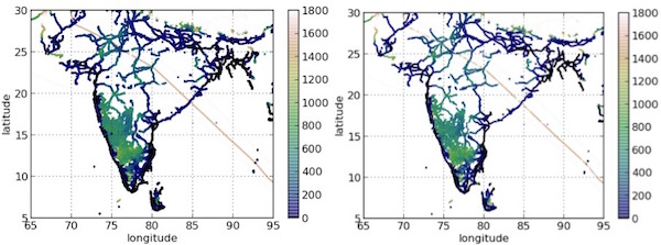
Figure 2 Original 2B-tuple dataset, visualized in 71 mins (left) and a 31M-tuple sample, visualized in 3 secs (right)
As you can see, the two plots are almost identical except that one takes 71mins to produce while the other takes only 3 seconds. This is because loading (and plotting) more data does not always improve the quality of the visualization. This occurs for many reasons:
- There are a finite number of pixels on your screen, so beyond a certain number of points, there is no difference.
- The human eye cannot notice any visual difference if it is smaller than a certain threshold.
- There is a lot of redundancy in most real-world datasets, which means a small sample of the entire dataset might lead to the same plot when visualized.
But I also want to clarify that you cannot just take a random (uniform) sample of the data and expect to produce high-quality visualizations. You need to use what we call visualization-aware sampling (VAS). This is how you can produce the plot above with only a tiny fraction of the entire data. There will be a separate post about how to create high-fidelity visualizations using just a tiny sample of the data.
3. Use AQP when your data is incomplete or noisy
Believe it not, most of the data that is collected and used in the real world is extremely noisy. So the idea that processing your entire data gives you 100% accurate answers is usually an illusion anyway. In other words, if my data is noisy to begin with, I might as well take advantage of approximation, which uses a controlled degree of noise in my computation in exchange for significant speed ups. This noise in your data can be because of many reasons:
- Human error: if humans have been involved in any part of your data entry process, your data is probably much noisier than you think. For example, patient records tend to have a lot of mistakes, typos, and inconsistencies, when they are manually entered by the medical staff.
- Missing values: Missing data is a major source of error. For example, if you insist on finding out the exact number of employees in your HR database who live within 5 miles of work, you should keep in mind that there are always people whose address is not up to date in your database.
- White noise: Even when your data is automatically collected, it can still have a lot of white noise. For example, sensor devices have a certain degree of noise. If your thermometer is recording 72 degrees, it is not always 100% accurate. Another example from click-log data is that you always have some small number of users who have clicked on an ad mistakenly.
- Data extraction errors: A lot of the data that is used for business intelligence is not handed to you in a proper format. In many cases, you have to use an extractor to crawl the web and extract the information you care about from various websites. These extractors introduce a lot of error too.
- Data conversion errors: When your data is a collection of various data sources, there is sometime a good deal of rounding and conversion errors. When the distance travelled is recorded as integer kilometers in one database and in integer miles in the another one, you have a little bit of conversion error for every record, which can add up to a lot of uncertainty when you look at the entire data.
In other words, in many situations, getting precise answers is nothing but an illusion: even when you process your entire data, the answer is still an approximate one. So why not use approximation to your computational advantage and in a way where the trade off between accuracy and efficiency is controlled by you?
4. Use AQP when your goal is to predict something
A lot of the time we don’t just query the data so that we can visualize thousands or millions of output results and then have an AHA moment. Instead, we query the data so that we can feed the output into a machine learning algorithm and make predictions, e.g., which ad is more likely to be clicked on by this user, what is the projected risk of an investment, and so on.
The majority of the commonly used techniques for inference are stochastic and probabilistic in nature. In other words, the predictions are based on a probabilistic analysis. In some cases, even the predictions themselves are probabilistic (e.g., in probabilistic classifiers). The good news is that these predictive models are designed to account for uncertainty and noise in their training data. This means adding a controlled degree of uncertainty to their input (e.g., by using approximate results) will not break their logic. In many cases, using a smaller sample of the data will lead to significant speedups with no or little impact on the accuracy of their predictions.
This is because the time complexity of many learning algorithms is super-linear (e.g., cubic or quadratic) in their input size, while the improvement of their learning curve has a diminishing return. Also, in some cases, certain forms of data reduction can even improve accuracy, e.g., by sampling down the majority class and creating a more balanced dataset for classification tasks. This is very common in online advertising, where there are far more visitors who do not click on an ad compared to those who do click. So when they use the web server logs to train a classifier (to decide which ad to show to each type of user) they first get rid of a lot of their non-clicking user logs to create more balanced training data. Another example is in linear regression, where a proper sample can be used to find a good approximate solution.***
In general, there are many cases where the output of the database queries are consumed by predictive analytics or machine learning algorithms, and in those cases, returning smaller samples of the original data can be a great solution for gaining considerable performance benefits.
I have enumerated a number of key use-cases where you should seriously consider approximate query processing if you are currently experiencing slow performance or are interested in reducing your Amazon AWS bills by an order of magnitude. There are other use-cases, such as billing or accounting, where you should NOT use approximation, because you probably won’t get away with it :)
Footnotes:
*, ** Miller, Robert B. "Response time in man-computer conversational transactions." Proceedings of the December 9-11, 1968, fall joint computer conference, part I. ACM, 1968.
*** A. Dasgupta, P. Drineas, B. Harb, R. Kumar, and M. W. Mahoney. Sampling algorithms and coresets for Lp
regression. SIAM Journal on Computing, 38, 2009.
Related Articles
- On HackerNews
- Strategy: Sample To Reduce Data Set
- Big Data Counting: How To Count A Billion Distinct Objects Using Only 1.5KB Of Memory
- Ask For Forgiveness Programming - Or How We'll Program 1000 Cores
- Approximate Query Processing: Taming the TeraBytes!
- CAP 6930: Approximate Query Processing
- Dynamic Sample Selection for Approximate Query Processing
- Tutorial on Sampling Theory for Approximate Query Processing