Cassandra NoSQL Data Model Design
This is a guest post by Ben Bromhead from Instaclustr

We at Instaclustr recently published a blog post on the most common data modelling mistakes that we see with Cassandra. This post was very popular and led me to think about what advice we could provide on how to approach designing your Cassandra data model so as to come up with a quality design that avoids the traps.
There are a number of good articles around that with rules and patterns to fit your data model into: 6 Step Guide to Apache Cassandra Data Modelling and Data Modelling Recommended Practices.
However, we haven’t found a step by step guide to analysing your data to determine how to fit in these rules and patterns. This white paper is a quick attempt at filling that gap.
Phase 1: Understand the data
This phase has two distinct steps that are both designed to gain a good understanding of the data that you are modelling and the access patterns required.
Define the data domain
The first step is to get a good understanding of your data domain. As someone very familiar with relation data modelling, I tend to sketch (or at least think) ER diagrams to understand the entities, their keys and relationships. However, if you’re familiar with another notation then it would likely work just as well. The key things you need to understand at a logical level are:
• What are the entities (or objects) in your data model?
• What are the primary key attributes of the entities?
• What are the relationships between the entities (i.e. references from one to the other)?
• What is the relative cardinality of the relationships (i.e. if you have a one to many is it one to 10 or one to 10,000 on average)?
Basically, these are the same things you’d expect in from logical ER model (although we probably don’t need a complete picture of all the attributes) along with a complete understanding of the cardinality of relationships that you’d normally need for a relational model. An understanding of the demographics of key attributes (cardinality, distribution) will also be useful in finalising your Cassandra model. Also, understand which key attributes are fixed and which change over the life of a record.
Define the required access patterns
The next step, or quite likely a step carried out in conjunction with step 1, is to understand how you will need to access your data:
- List out the paths you will follow to access the data, such as:
- Start with a customer id, search for transactions in a date range and then look up all the details about a particular transaction from the search resultsStart with a particular server and metric, retrieve x metrics values in ascending age
- Start with a particular server and metric, retrieve x metrics values in ascending age starting at a particular point in time.
- For a given sensor, retrieve all readings of multiple metrics for a given day.
- For a given sensor, retrieve the current value.
- Remember that any updates of a record are an access path that needs to be considered
- Determine which accesses are the most crucial from a performance point of view – are there some which need to be as quick as possible while performance requirements for others allow time for multiple reads or range scans?
- Remember that you need a pretty complete understanding of how you will access your data at this stage – part of the trade-off for Cassandra’s performance, reliability and scalability is a fairly restricted set of methods for accessing data in a particular table.
Phase 2: Understand the entities
This phase has two specific steps designed to gain an understanding of both the primary and secondary entities associated with the data.
Identify primary access entities
Now we’re moving from analysing your data domain and application requirements to starting to design your data model. You really want to be pretty solid on steps 1 and 2 before moving on to this stage.
The idea here is to denormalize your data into the smallest number of tables possible based on your access patterns. For each lookup by key that your access patterns require, you will need a table to satisfy that lookup. I’ve coined the term primary access entity to describe the entity your using for the lookup (for example, a lookup by client id is using client as the primary access entity, a lookup by server and metric name is using a server-metric entity as the primary access entity).
The primary access entity defines the partition level (or grain if you’re familiar with dimensional modelling) of the resulting denormalized table (i.e. there will be one partition in the table for each instance of the primary access entity).
You may choose to satisfy some access patterns using secondary indexes rather than complete replicas of the data with a different primary access entity. Keep in mind that columns in include in a secondary index should have a significantly lower cardinality than the table being indexed and be aware of the frequency of updates of the indexed value.
For the example access patterns above, we would define the following primary access entities:
- customer and transaction (get a list of transactions from the customer entity and then use that to look up transaction details from the transaction entity)
- server-metric
- sensor
- sensor
Allocate secondary entities
The next step is to find a place to store the data that belongs to entities that have not been chosen as primary access entities (I’ll call these entities secondary entities). You can choose to:
- Push down by taking data from a parent secondary entity (one side) of a one to many relationship and storing multiple copies of it at the primary access entity level (for example, storing customer phone number in each customer order record); or
- Push up by taking data from the child secondary entity (many side) of a one to many relationship and storing it at the primary access entity level either by use of cluster keys or by use of multi-value types (list and maps) (for example adding a list of line items to a transaction level table).
For some secondary entities, there will only be one related primary access entity and so there is no need to choose where and which direction to push. For other entities, you will need to choose will need to choose which primary access entities to push the data into.
For optimal read performance, you should push a copy of the data to every primary access entity that is used as an access path for the data in the secondary entity.
However, this comes at an insert/update performance and application complexity cost of maintaining multiple copies the data. This trade-off between read performance and data maintenance cost needs to be judged in the context of the specific performance requirements of your application.
The other decision to be made at this stage is between using a cluster key or a multi-value type for pushing up. In general:
- Use a clustering key where there is only one child secondary entity to push up and particularly where the child secondary entity itself has children to roll-up.
- Use multi-value types where there are multiple child entities to push up into the primary entity
Note that these rules are probably oversimplified but serve as a starting point for more detailed consideration.
Phase 3: Review & Tune
The last phase provides an opportunity to review the data model, test and to tune as necessary.
Review partition & cluster keys
Entering this stage, you have all the data you need to store allocated to a table or tables and your tables support accessing that data according to your required access patterns. The next step is to check that the resulting data model makes efficient use of Cassandra and, if not, to adjust. The items to check and adjust at this stage are:
- Do your partition keys have sufficient cardinality? If not, it may be necessary to move columns from the clustering key to the partition key (e.g. changing primary key (client_id, timestamp) to primary key ((client_id, timestamp))) or introduce new columns which group multiple cluster keys into partitions (e.g. changing primary key (client_id, timestamp) to primary key ((client_id, day), timestamp).
- Will the values in your partition keys be updated frequently?Updates of a primary key value will result in deletion and re-insertion of the record which can result in issues with tombstones. For example, trying to maintain a table with all clients of a particular status, you might have primary key (status, client ID). However, this will result in a delete and re-insert every time a client’s status changes. This would be a good candidate to use a set or list data type rather than including client ID as the cluster key.
- Is the number of records in each partition bounded? Extremely large partitions and/or very unevenly sized partitions can cause issues. For example, if you have a client_updates table with primary key (client_id, update_timestamp) there is potentially no limit to how many times a particular client record can be update and you may have significant unevenness if you have a small number of clients that have been around for 10 years and most clients only having a day or two’s history. This is another example where it’s useful to introduce new columns which group multiple cluster keys into partitions partitions (e.g. changing primary key (client_ id, update_timestamp) to primary key ((client_id, month), update_timestamp).
Test and tune
The final step is perhaps the most important – test your data model and tune it as required. Keep in mind that issues like partitions or rows growing too large or tombstones building up in a table may only become visible after days (or longer) of use under real-world load. It’s therefore important to test as closely as possible to real-world load and to monitor closely for any warning signs (the nodetool cfstats and cfhistograms commands are very useful for this).
At this stage you may also consider tuning some of the settings that effect the physical storage of your data. For example:
- changing compaction strategy;
- reducing gc_grace_seconds if you are only deleting data using TTL; or
- setting caching options.
A Worked Example
To illustrate this, I’ll walk through a basic example based on building a database to store and retrieve log messages from multiple servers. Note this is quite simplified compared to most real-world requirements.
Step 1: Define the data domain

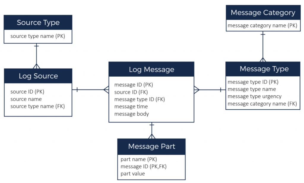
The previous ER diagram illustrated the data domain. We have:
- Lots (millions) of log messages which have a timestamp and a body. Although message ID is shown as the primary key in the ER diagram, message time plus message type is an alternate primary key.
- Each log message has a message type and types are further grouped into a message category (for example, a message type might be “out of memory error” and category might be “error”). There a couple of hundred message types and around 20 categories.
- Each log message comes from a message source. The message source is the server that generated the message. There are 1000s of servers in our system. Each message source has a source type to categorise the source (e.g. red hat server, ubuntu server, windows server, router, etc.). There are around 20 source types. There are ~10,000 messages per source per day.
- The message body can be parsed and stored as multiple message parts (basically key, value pairs). There is typically less than 20 parts per message.
Step 2: Define the required access patterns
We need to be able to:
- Retrieve all available information about the most recent 10 messages for a given source (and be able to work back in time from there).
- Retrieve all available information about the most recent 10 message for a given source type.
Step 3: Identify primary access entities
There are two primary access entities here – source and source type. The cardinality (~20) of source type makes it a good candidate for a secondary index so we will use source as the primary access entity and add a secondary index for source type.
Step 4: Allocate secondary entities
In this example, this step is relatively simple as all data needs to roll into the log source primary access entity. So we:
- Push down source type name
- Push down message category and message type to log message
- Push up log message as the clustering key for the new entity
- Push up message part as a map type with.
The end result is that would be a single table with a partition key of source ID and a clustering key of (message time, message type).
Step 5: Review partition and cluster keys
Checking these partition and cluster keys against the checklist:
- Do your partition keys have sufficient cardinality? Yes, there are 1000s of sources.
- Will the values in your partition keys being updated frequently? No, all the data is write-once.
- Is the number of records in each partition bounded? No – messages could build up indefinitely over time.
So, we need to address the unbound partition size. A typical pattern to address that in time series data such as this is to introduce a grouping of time periods into the cluster key. In this case 10,000 messages per day is a reasonable number to include in one partition so we’ll use day as part of our partition key.
The resulting Cassandra table will look some like:
|
1
2
3
4
5
6
7
8
9
10
11
12
13
14
15
16
17
|
CREATE TABLE example.log_messages (
message_id uuid,
source_name text,
source_type text,
message_type text,
message_urgency int,
message_category text,
message_time timestamp,
message_time_day text,
message_body text,
message_parts map<text, frozen >
PRIMARY KEY ((source_name, message_time_day,
message_time, message_type)
) WITH CLUSTERING ORDER BY (message_time DESC);
CREATE INDEX log_messages_sourcetype_idx ON
example.log_messages (source_type);
|
Conclusion
Hopefully, this process and basic example will help you start to get familiar with Cassandra data modelling. We’ve only covered a basic implementation that fits well with Cassandra, however there are many other examples on the web which can help you work through more complex requirements. Instaclustr also provides our customers with data modelling review and assistance, so get in touch with us if you need some hands-on assistance.


