Designing Uber

This is a guest post by Ankit Sirmorya. Ankit is working as a Machine Learning Lead/Sr. Machine Learning Engineer at Amazon and has led several machine-learning initiatives across the Amazon ecosystem. Ankit has been working on applying machine learning to solve ambiguous business problems and improve customer experience. For instance, he created a platform for experimenting with different hypotheses on Amazon product pages using reinforcement learning techniques. Currently, he is in the Alexa Shopping organization where he is developing machine-learning-based solutions to send personalized reorder hints to customers for improving their experience.

Requirements

In Scope

• Riders should be able to view the available drivers in nearby locations as shown in the image below.
  

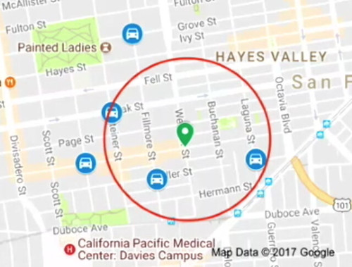
Fig: Showing nearby car locations

• Riders should be able to request rides from source to destination.
• Nearby drivers will be notified of the ride, and one of them will confirm the ride
• Pickup ETA will be shown to customers when a ride is dispatched to pick up the rider.
• Once the trip gets completed, the rider is shown the trip details such as the trip map, price, and so forth in the ride receipt.

Out of Scope

• Automated way of matching drivers to riders taking factors such as new drivers and riders into account when a ride is being dispatched

Architecture

In order to design the system, it’s imperative to define the lifecycle of a trip, shown in the image below.

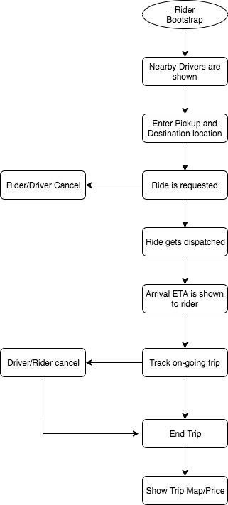
Fig: Lifecycle of a trip

We can build the following components to support this trip lifecycle. These components will work together to meet the requirements of building a ride-hailing system.

• Driver Location Manager: This component will be responsible for maintaining the changing driver locations. It will ingest the messages emitted by the drivers' uber app containing their current locations and update the car location index.
• Trip Dispatcher: It will be responsible for handling the trip requests from users and dispatch a driver in response to those requests.
• Arrival ETA Calculator: This component will be responsible for calculating the ETA for the driver to reach the rider once the driver has accepted the ride.
• Trip Recorder: It will record the GPS signals transmitted from the ride when the trip is in progress. These GPS signals will then be recorded in a data store which will be used by subsequent systems such as Map Matcher and Pricing Calculator.
• Map Matcher: This component will be responsible for matching the trip on the actual map using algorithms specialized for this purpose.
• Price Calculator: It will use the recorded trip information for computing the price which users have to pay for the trip.

The components mentioned above can be grouped into three major categories: Pre-Trip Components, On-Trip Components, and Data Storage. We have shown each of the components in the image below.

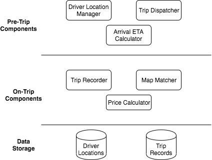
Fig: High-level components in a ride hailing system

High Level Design

Pre-Trip Component

This component will be supporting the functionality to see the cars in the nearby locations and dispatching the ride on users’ requests. The location of the cars can be stored in an in-memory car location index (explained in a later section), which can support high read and write requests. The driver app will keep on sending the updated car locations, which will be updated in this index. The index will be queried when rider app requests for nearby car locations or places a ride request. The sequence of operations leading to the ride dispatch is shown in the image below.

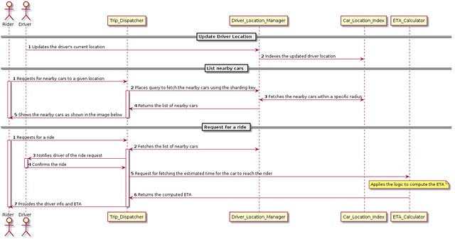
Fig: Sequence of Operations in the Pre-Trip Component

There are three sequences of operations before a trip starts, as shown in the image above: i) Update Driver Location ii) List nearby drivers iii) Requesting for a ride. The first sequence of operations involves updating the driver locations as drivers keep changing their locations. The second sequence comprises of the steps involved in fetching the list of nearby drivers. The third sequence includes a series of steps involved in requesting and dispatching a ride.

Car Location Index

We will maintain the driver locations in a distributed index, which is spread across multiple nodes. The driver information containing their locations, the number of people in the car, and if they are on a trip is aggregated as objects. These driver objects are distributed across the nodes using some sharding mechanism (e.g., city, product, and so forth) along-with replication.

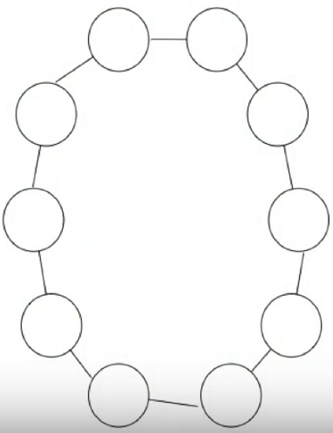
Fig: Distributed Car Location Index

Each node maintains a list of drivers objects which are queried in real-time to fetch the list of nearby drivers. On the other hand, these objects are updated when the driver app sends updates about their location or any other related information. Some interesting characteristics of this index are listed below.

• It should store the current locations of all drivers and should support fast queries by location and properties such as driver’s trip status.
• It should support a high volume of reads and writes.
• The data stored in these indexes will be ephemeral, and we don’t need long-term durable storage.

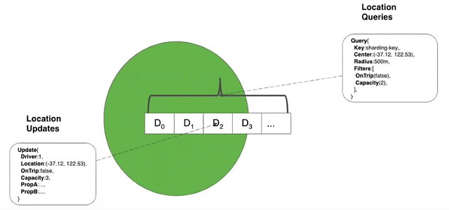
Fig: Updating and Querying Car Location Index

ETA Calculator

We need to show the pickup ETA to users once their ride has been dispatched by taking factors such as route, traffic, and weather into account. The two primary components of estimating an ETA given an origin and destination on a road network include i) computing the route from origin to destination with the least cost (which is a function of time & distance) ii) estimate the time taken to traverse the route.

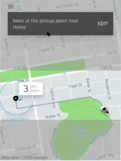
Fig: Sample ETA shown to customer

We can start by representing the physical map by a graphical representation to facilitate route computation. We do this by modeling every intersection by node and each road segment by a directed edge. We have shown the graphical representation of the physical map in the image below.

Fig: Graph Representation of physical map

We can use routing algorithms such as Dijkstra’s algorithm to find the shortest path between source and destination. However, the caveat associated with using Dijkstra’s algorithm is that the time to find the shortest path for “N” nodes is O(NlgN) which renders this approach infeasible for the scale at which these ride hailing platforms function. We can solve this problem by partitioning the entire graph, pre-computing the best path within partitions, and interacting with just the boundaries of the partitions. In the image below, we have shown the manner in which this approach can help in significantly reducing the time complexity from O(NlgN) to O(N’lgN’), where N’ is square root of N.

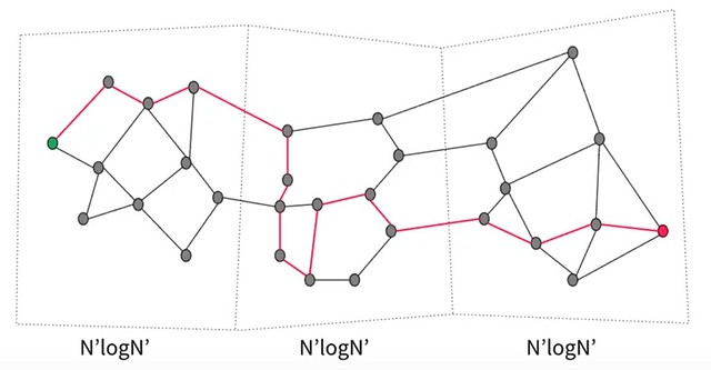
Fig: Partitioning Algorithms to find the optimal route

Once we are aware of the optimal route we find the estimated time to traverse the road segment by taking traffic into account which is a function of time, weather and real-life events. We use this traffic information to populate the edge weights on the graph, as shown in the image below.

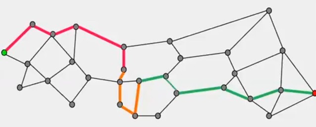
Fig: Using traffic information to determine ETA

On-Trip Component

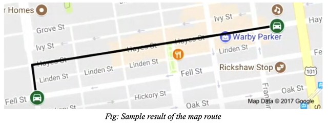
This component handles the processes which are involved from start to completion of the trip. It keeps track of the locations of the ride when the trip is in progress. It also is responsible for generating the map route (shown in image below) and computing the trip cost when it gets completed.

In the image below, we have shown the sequence of operations which are involved while the trip is in progress and also when it has completed. The driver app publishes GPS locations when the ride is in progress which is consumed by the Trip Recorder through Kafka streams and persisted in the Location Store. Upon trip completion, Map Matcher generates the map route using the raw GPS locations.

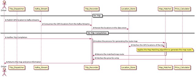
Fig: Sequence Diagram for On Trip Components

Location Store/Data Model

This storage component will be responsible for storing the stream of GPS locations sent by the rider/driver app while the trip is in progress. Some of the characteristics of this store are listed below.

• It should support high volume of writes.
• The storage should be durable.
• It should support timeseries based queries such as the location of driver in a given time range.

We can use a datastore such as Cassandra for persisting the driver locations, thereby, ensuring long-term durability. We can use a combination of  as the partition key for storing the driver locations in the data store. This ensures that the driver locations are ordered by timestamp and can support time-based queries. We can store the location point as serialized message in the data store.

Map Matcher

This module takes in raw GPS signals as input and outputs the position on road network. The input GPS signals comprises of latitude, longitude, speed and course. On the other hand, the positions on a road network comprises of latitude (on an actual road), longitude (on an actual road), road segment id, road name, and direction/heading. This is an interesting challenge in itself as the raw GPS signals can be far away from the actual road network. Few such examples are shown in the image below where the box on the top-left corresponds to an urban canyon situation caused by tall buildings and the one in the bottom-right is due to sparse GPS signals. The map route generated by Map Matcher is used for two major use-cases: i) finding the actual position of the driver on the road network ii) calculating the fare prices.

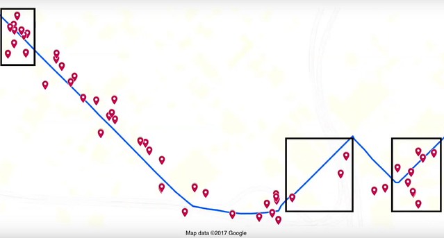
Fig: Challenges of Map Matching: Urban Canyon, Sparse GPS Signals

To solve the Map Matching problem, we need to determine the route which the car would have taken while being on the trip. We can use the approach of Hidden Markov Model (HMM) to find globally optimal route (collection of road segments; i.e. R1, R2, R3, …) which the car would have taken based on the observed GPS signals (O1, O2, O3, …). In the image below, we have shown a sample representation of road segments and GPS signals.

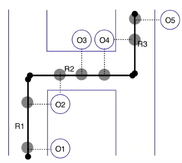
Fig: Sample of GPS signals and road segments

After that, the GPS signals and road segments are represented using Hidden Markov Model (HMM) using Emission Probability (probability of observing a GPS signal from a road segment) and Transition Probability (probability of transitioning from one road segment to another). We have explained this scenario in the image by modeling road segments as hidden states and GPS signals as observations using HMM.

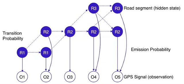
Fig: Representing GPS signals and road segments using HMM

We can then apply dynamic programming-based Viterbi algorithm on an HMM to find the hidden states given a set of observations. We have shown the output of Viterbi algorithm after running it on the HMM we have discussed in this example.

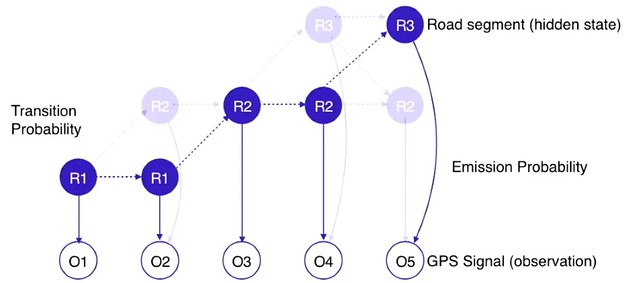
Fig: Output of Viterbi algorithm after running it on the HMM mentioned above

Optimizations

One of the problem with the proposed design is that both the heavy reads and writes are directed to the data store. We can optimize the system by separating the read traffic from the writes by caching the raw driver locations in a distributed cache (Redis). The raw driver locations from the Redis cache is leveraged by MapMatcher to create the matched map and persist it in the data-store.

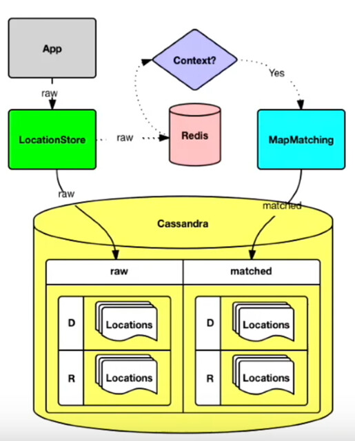
Fig: Optimization to offload the reads from Cassandra to Redis Cache

We can also improve the predicted ETAs by applying machine learning on top of the ETA calculation mechanism mentioned above. The first challenge of applying machine learning involve feature engineering to come up with features such as region, time, trip type, and driver behavior to predict realistic ETAs. Another interesting challenge would be to select the machine learning model which can be used for predicting the ETAs. For this use-case, we would rely on using a non-linear (e.g. ETA doesn’t linearly relate with hour of the day) and non-parametric (there is no prior information on interaction between different features and ETA) model such as Random Forest, Neural networks and KNN learning. We can further improve the ETA prediction by monitoring customer issues when the ETA prediction is off.

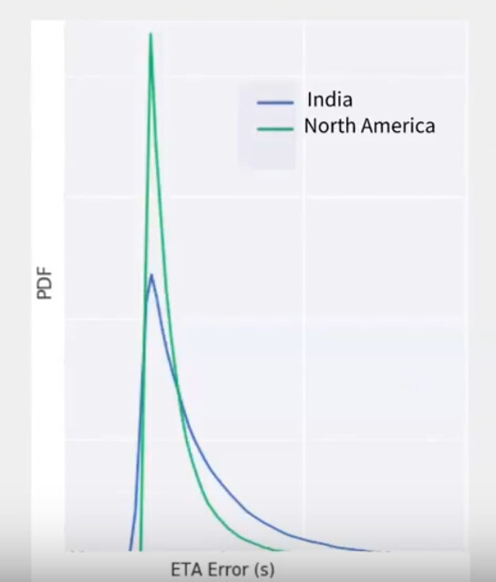
FUN FACT: In this talk, data scientist Sreeta Gorripaty @ Uber, has discussed about the correlation between ETA error(actual ETA – predicted ETA) and region. As part of Feature Engineering, the probability density function (PDF) of the ETA error is shown in the graph below. The graph shows that the distribution has thicker tails in India compared to North America. It indicates that the ETA predictions are worse in India, making region an important feature for training the machine learning model which is used for ETA prediction

Addressing Bottlenecks:

In the system, each of the components comprise of different micro-services each performing a separate task. We will be having separate web-services for Driver Location Management, Map Matching, ETA calculation and so forth. We can make the system more resilient by having fallback mechanism in-place to account for service failures. Some common fallback mechanisms include using the most recently cached data or even using fallback web-services in some cases. Chaos engineering is a commonly used approach for resiliency testing where failures/disruptions are injected in the system and its performance is monitored to make improvements for making the service more resilient to failures.

In the image below, we have shown the architecture of the Chaos Platform which can be used for introducing disruptions/failures in the system and monitoring those failures on dashboards. The failures are introduced by developers through command line arguments by passing the disruption configurations in a file. The worker environments in the Chaos platform trigger the agents in the hosts to create failures using the configurations passed as input. These workers maintain the disruption logs and events through streaming RPC and persist that information in database.

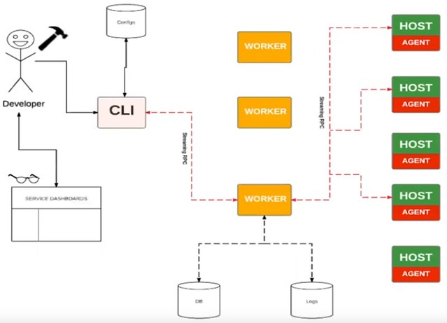
Fig: Chaos Platform @ Uber

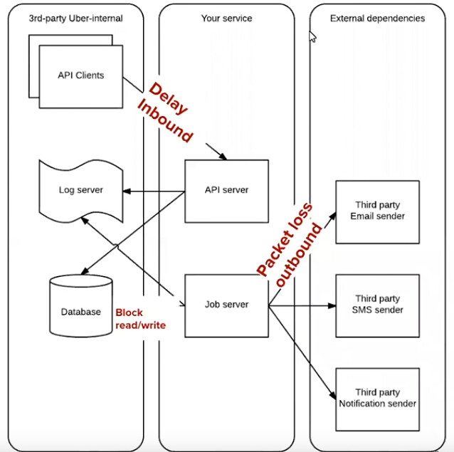
We can introduce two types of disruptions for the purpose of resiliency testing. The first kind of failures are called the process-level failures such as SIGKILL, SIGINT, SIGTERM, CPU throttling, and Memory limiting. The second type of failures are the Network-level failures such as Delays in the inbound network calls, Packet Loss in the outbound calls to the external dependencies, and blocking read/writes to the database. We have shown all the different kind of network failures in the image below.

Extended Requirement:

In the design above, the drivers were being notified of the nearby riders and they were accepting the rides they wanted. As an extension of the existing implementation, the interviewer may ask to extend the system to enable automated matching of drivers to riders. The drivers are matched to riders based on factors such as the distance between drivers and riders, direction in which the driver is moving, traffic and so forth. We can apply the naïve approach of matching riders to the nearest driver. However, this approach doesn’t tackle the problem of something called trip upgrade which occurs when a rider is matched to a driver and at the same time an additional driver and an additional rider enters the system. The trip upgrade scenario is illustrated in the images below.

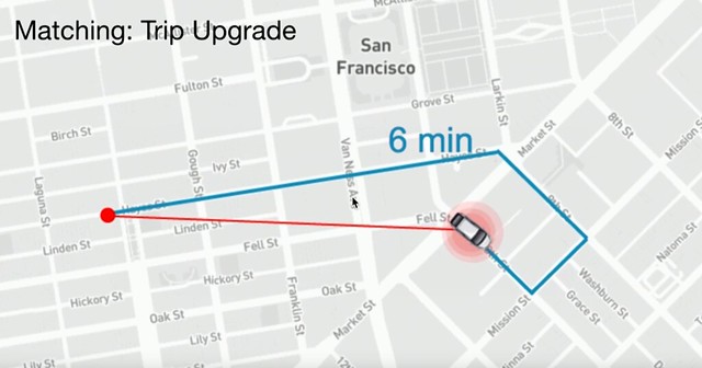
Fig: Trip Upgrade - Rider gets matched to a driver

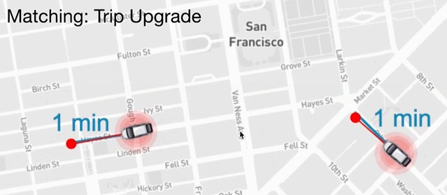
Fig: Trip Upgrade - Additional Driver and Rider enters the system

FUN FACT: Dawn Woodard, Uber’s senior data science manager of maps, has talked about the science behind the Matching @Uber in her talk at Microsoft Research.  Dawn has talked about different methods for matching and dynamic pricing in ride-hailing, and discussed machine learning and statistical approaches used to predict key inputs into those algorithms: demand, supply, and travel time in the road network.

References

• Backend of Requesting Ride(Arka) https://www.youtube.com/watch?v=AzptiVdUJXg
• Mapping(Kiran) https://www.youtube.com/watch?v=ChtumoDfZXI
• ETA Calculation: https://www.youtube.com/watch?v=FEebOd-Pdwg
• Uber Payments: https://www.youtube.com/watch?v=Dz6dAZs8Scg
• Life of a Trip: https://youtu.be/GyS3m5SyRuQ?list=PLLEUtp5eGr7DcknAkGa62w4LmyAfz37Au&t=123